Implementing “Tennis for Two” using op amps

“Tennis for Two” is the name given to an early video game implemented on an analog computer. See https://en.wikipedia.org/wiki/Tennis_for_Two and https://en.wikipedia.org/wiki/Early_history_of_video_games for more information on the game itself. This post documents the construction of a “Tennis for Two”-like game using op amps.

For the impatient 1: jump to the video section

For the impatient 2: jump to the schematics

Some references

Mubarik Mohamoud “The Bouncing ball analog computer” (PDF)

https://www.analogmuseum.org/english/examples/bouncing_ball/ (Great site)

Heathkit EC-1 manual (PDF) (this manual itself lists a lot of references to books from the 1950s, most of which seem to be available on archive.org! If you’re into that kind of thing.) It looks like this manual already contains a bouncing ball circuit; a lot of people seem to be under the impression that Telefunken were the first to have such a circuit in their manual.

Look Mum No Computer – Bouncing Balls With DIY Electric Analog Circuits (YouTube)

Introduction

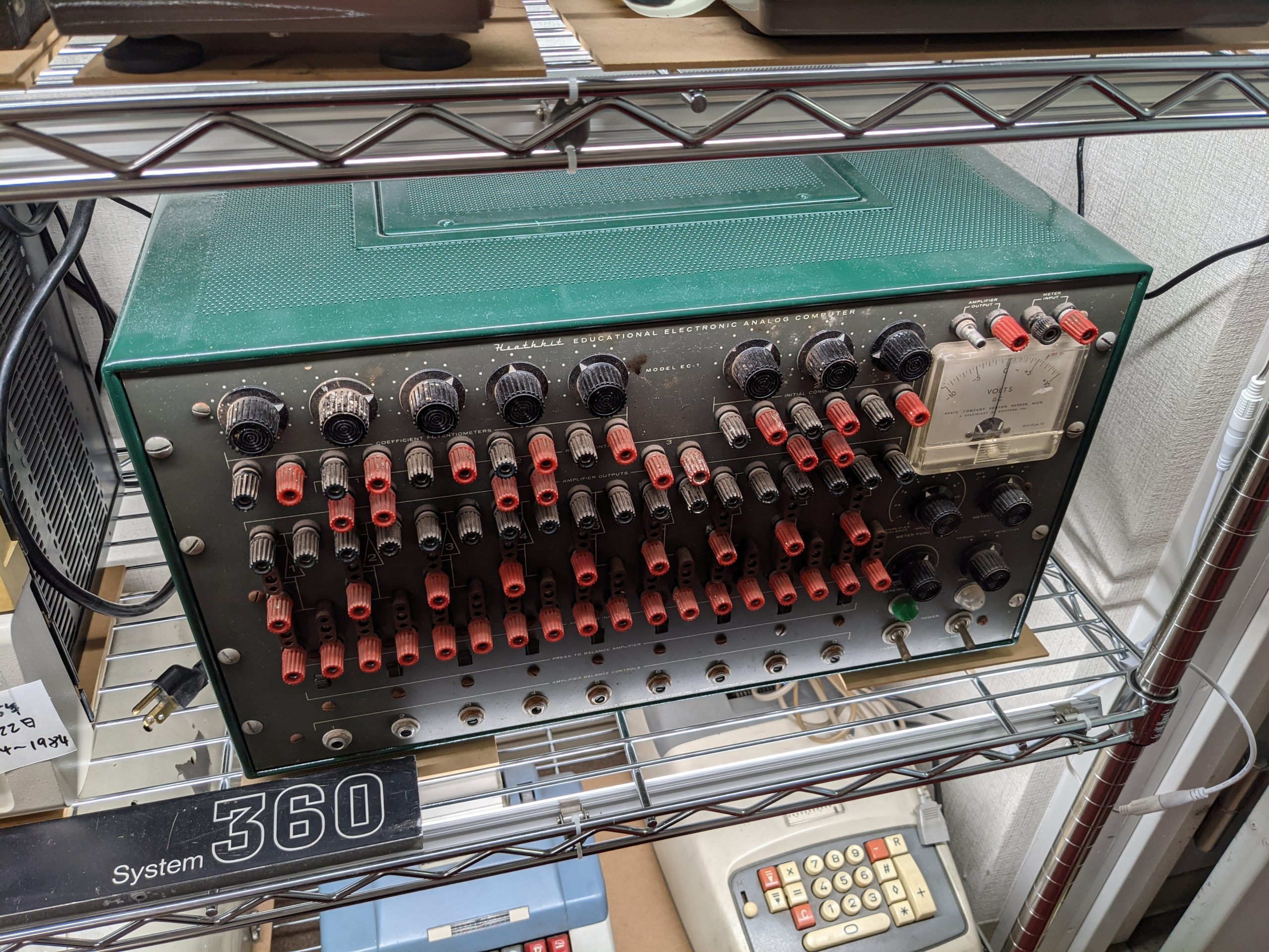
Analog computers were a thing, a long time ago. What do they do? They basically consist of a power supply, a breadboard-like area, a bunch of potentiometers to set input values, and a bunch of op amps in various configurations. The breadboard-like area would (for example) be color-coded and the user would attach jumper cables between different color-coded areas. However, back in the day, op amps weren’t tiny ICs that could be had for the price of a paper airplane folded out of old newspaper. They were discrete, and made of vacuum tubes (when they were invented in 1941), or, after transistors became available, discrete transistors.

Using analog computers (and op amps), you could, for example, sum voltages, invert voltages, and integrate and differentiate voltages over time. Let’s try and remember some calculus from high school or university and recall what differentiating and integrating means.

If you don’t have any basic knowledge of op amps yet, EEVBlog has a good video explaining the basics at https://www.youtube.com/watch?v=7FYHt5XviKc. It isn’t absolutely necessary to understand the basic concepts of op amps, you can just use them as “black box” integrators.

Some math

If you don’t remember much with regards to differentiation and integration, skip to the next paragraph. If you remember a bit more, here’s the ultra-condensed version of the below explanation:
Differentiating a curve gets us a straight line, differentiating a straight line gets us a constant. Integration is the opposite of differentiation, so disregarding some lossy bits, integrating the constant gets us the straight line again. Integrating the straight line gets us the curve again. We can easily set a constant voltage using a potentiometer, and we can easily integrate using op amps.

Now, the less condensed version: here is a random list of facts that you may or may not remember:

1. Integrating is the opposite of differentiation (that’s the easy one)
2. Differentiation means getting the slope of a curve
3. Integration, being the opposite of differentiation, means that we get the curve from the slope (a slightly lossy operation, as there is more than one curve with the same slope)
4. You can differentiate things more than once. For example, from a quadratic curve (e.g., f(x)=x²) the first derivative yields a straight line (f'(x)=2x), from the straight line you get a constant (f”(x)=2). Integrating can be done more than once too, and as mentioned before, is the other way round, so from a constant you get a straight line, from the straight line you get a quadratic curve.

Now let’s say we have some acceleration, like… for example 9.8 m/s².
(There is a planet called Earth in the Milky Way, named after the fact that some of its crust consists of earth. The same type of earth as you’d find in a potted plant. When you drop objects from a small height onto this planet, they accelerate, and the rate of acceleration is 9.8 m/s². 9.8 is very close to π² and this is not a coincidence. Also the people who live there are made of meat, but that’s a topic for another day.)
So after 1 second the dropped object has a speed of 9.8 m/s, and after two seconds it’s 19.6 m/s, etc. Dropped objects get faster and faster. If you plot the speed of the object, you get a linear (i.e. straight) graph. However, if you plot the distance of the object from the point it was dropped, you get a curve, i.e., it gets steeper and steeper.

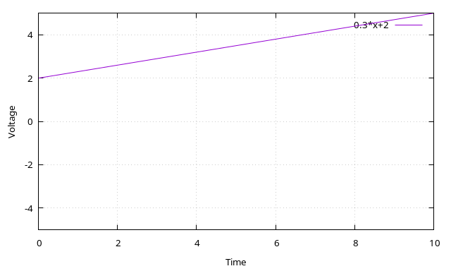
Let’s say, all we have at first is a constant, 9.8. In math terms, we could say that the function always producing this constant is f”(x)=9.8. (I added two apostrophes to “foreshadow” that we will be integrating this twice.) To get a linear function from the constant, we can integrate. The mathematical result of the integration is f'(x)=9.8x (+ some constant, which we will ignore here and below). Don’t remember enough about this to believe me? Try https://www.wolframalpha.com/input?i=integrate+9.8

This would draw a line with a rather steep gradient of 9.8. Implemented using op amps, the integrating op amp will have 9.8V on the input side, and a voltage linearly going up on the output. (Note: the op amp will invert the input, so in reality the voltage will go down, but that is not a major problem.)

To get a function that would plot as a curve from this linear function, we integrate again using a second op amp, and the result will be the function f(x)=4.9x² (ask Wolfram Alpha if you don’t remember how to do this (“integrate 9.8x”)). Now check out the formula to get the distance fallen after a time of t seconds at https://en.wikipedia.org/wiki/Equations_for_a_falling_body#Equations:

Hey, that’s exactly the same formula! (g is 9.8, 1/2*g is 4.9, and t is just a rename of x.)

(Done with the math, time to talk about some electronics)

On an oscilloscope, the Y axis is voltage and the X axis is just “time”. Oscilloscopes commonly offer another mode, the X-Y mode. In this mode, one channel’s voltage will be plotted on the X axis, and another channel’s voltage on the Y-axis. Using this mode, we can simulate the effects of gravity on the Y axis and the horizontal movement of a tennis ball on the X axis. (Of course, the X-Y mode won’t exactly make it easy to debug things, so for now we’ll mostly work in the regular mode.)

Just a few more notes and we’re ready to implement stuff on breadboards and start looking at the resulting signals on an oscilloscope!

• The power supply needs to generate a negative voltage, 0V, and a positive voltage. I’m using an old ATX power supply that I bought at a thrift store and have -5V/5V as well as -12V/12V. I use -5/5V below, this makes it much easier to interface with other components. If you don’t have anything fancy, you can just use two 5V wall warts back-to-back, or a couple AA batteries in series and tapped in the middle, or whatever you want!
• Constants are just arbitrary voltages input using potentiometers. We don’t have to use 9.8V, we’ll just use something that is convenient and looks okay.
• To integrate an input signal using an op amp, all we need to do is put a capacitor between the input and the output of the op amp. We’ll also need a resistor to make the integration happen non-instantaneously. (Check https://en.wikipedia.org/wiki/Op_amp_integrator or similar to learn more)
• The op amp’s output will be inverted
• To make the integration slow enough, we need capacitors with a high capacitance. But preferably we don’t want to have to take capacitor polarization into account, so we won’t use electrolytic capacitors. I’ll be using a 1 μF ceramic capacitor, which is the highest non-polarized capacitor value I have and makes our calculations very easy. We’ll also need resistors with a high resistance in the MΩ range, as the RC delay when using a 1 MΩ resistor with a 1 μF capacitor is 1 second (1000000 x 0.000001 = 1).

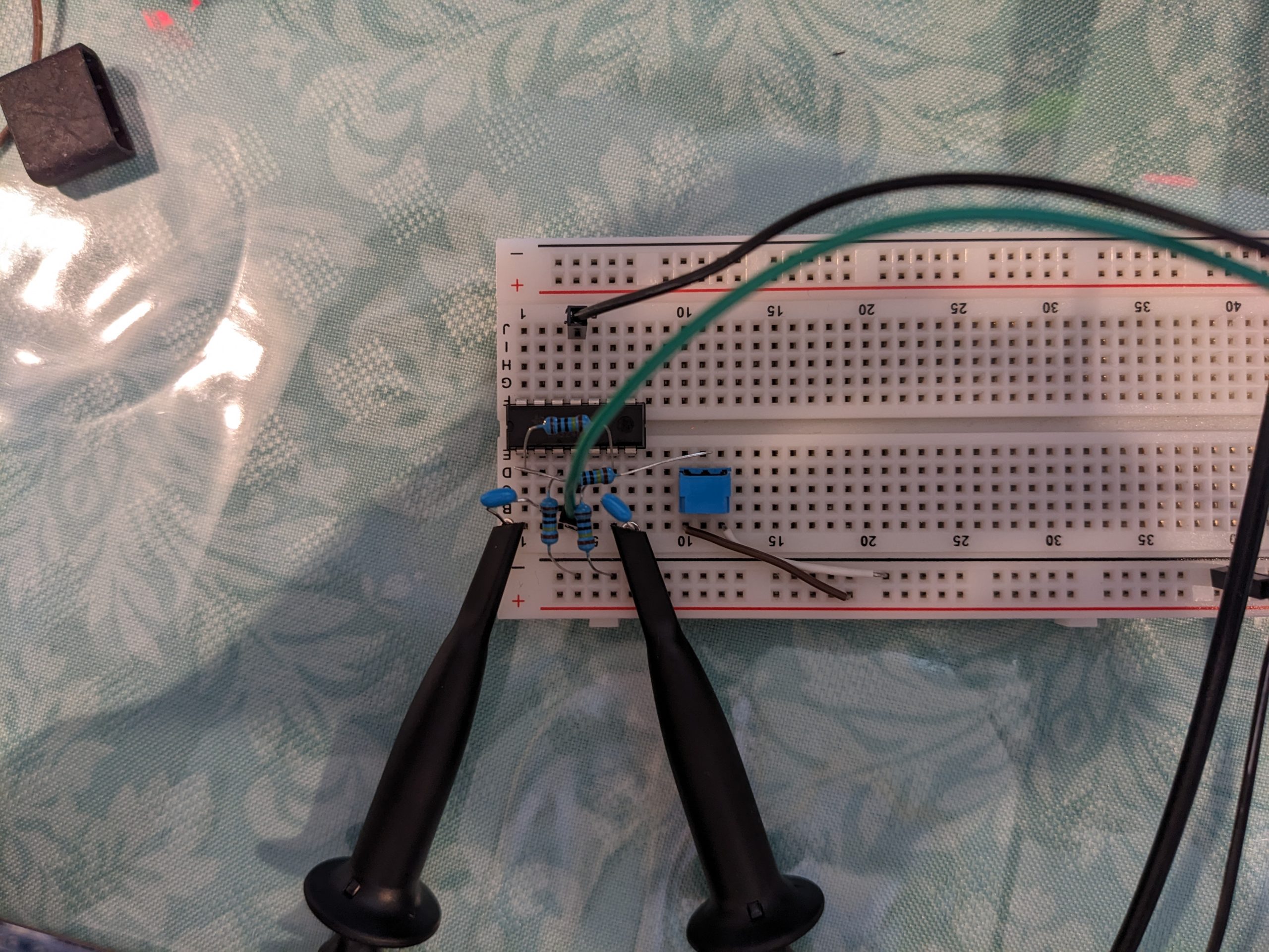
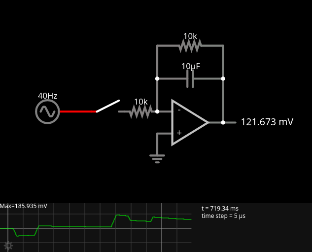
To get started, here’s the setup with an op amp integrating our constant fed in using a potentiometer:

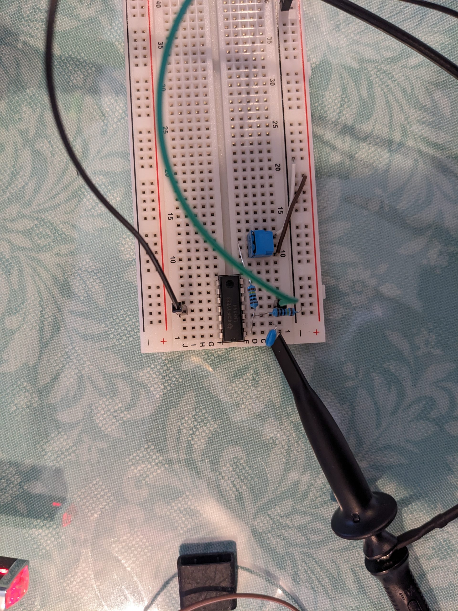
In this circuit, I’m using an LM324N quad op amp. The pinout looks like this:

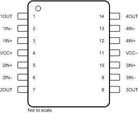
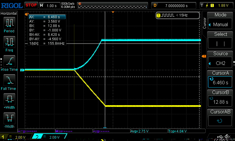
And here’s what we get on our oscilloscope:

Let’s integrate that straight line again. Here’s our setup:

And here’s what we see on the oscilloscope (probing the previous output stage and this output stage at the same time):

Is that all there is to the Y axis? Well, no. First of all, we are currently falling “up”. That’s easily fixed; we could just invert the signal again using another op amp. Or maybe we could simply input a negative voltage as our gravity, then we wouldn’t need to use an extra op amp circuit? Let’s not worry about that for now, we have some other things to take care of. Remember, this game/simulation is supposed to be tennis-like.

Tennis balls should bounce off the floor. Oh right, we don’t even have a “floor” yet, per se. We see that both signals reach “a floor” or “ceiling”, but they’re actually just reaching the op amp’s voltage rails (-5V and 5V) or the voltage set by the potentiometer, at which point they can’t go any further.

To make the ball bounce, we can “override” the gravity input and quickly feed in a negative voltage instead. (Of course, the gravity input is still there, just with a much higher resistance.) Conveniently, our floor is a negative voltage. (In the above pic, we’re still inverted of course. If we add another op amp, we can invert this signal.) We just need to “copy” this voltage to the – input of the very first op amp and we’ll produce a beautiful bounce. (“Cool so we just write some code and copy some variables, right.” “Wrong, sit down!”)

One immensely popular way to copy a voltage from one place to another is to use a wire to connect the two places! But in our case, we want a smart wire. This wire shouldn’t be active until we reach the floor (which is just a certain negative voltage of our choosing). Well, it may not be immediately obvious, but one of the most famous components in the world of electronics happens to have this property! We have surely heard of diodes before, right? A single standard diode doesn’t become active until we reach 0.7 V. If we use two diodes, it’s 1.4V, three diodes, 2.1V, etc. If we have negative voltages, we just flip the diode’s terminals around. Cool! But inconvenient. Here’s another type of diode though: the zener diode. Zener diodes are designed to be reverse-biased and become conductive (generally, very suddenly) at a certain voltage. So instead of (e.g.) stacking four regular diodes, we could use a single zener diode with a breakdown voltage of approximately 2.8V (and flip its poles because it’s reverse-biased).

So we just connect the output of the third op amp back to the input of the first op amp, via a diode!

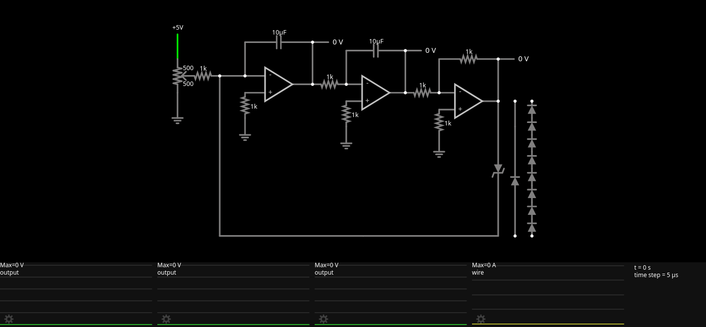
Well, things don’t look too bad in this simulation! Currently, the ball just bounces back to its previous level, but we could easily add a little something to dampen the voltage, which I may or may not explain later:

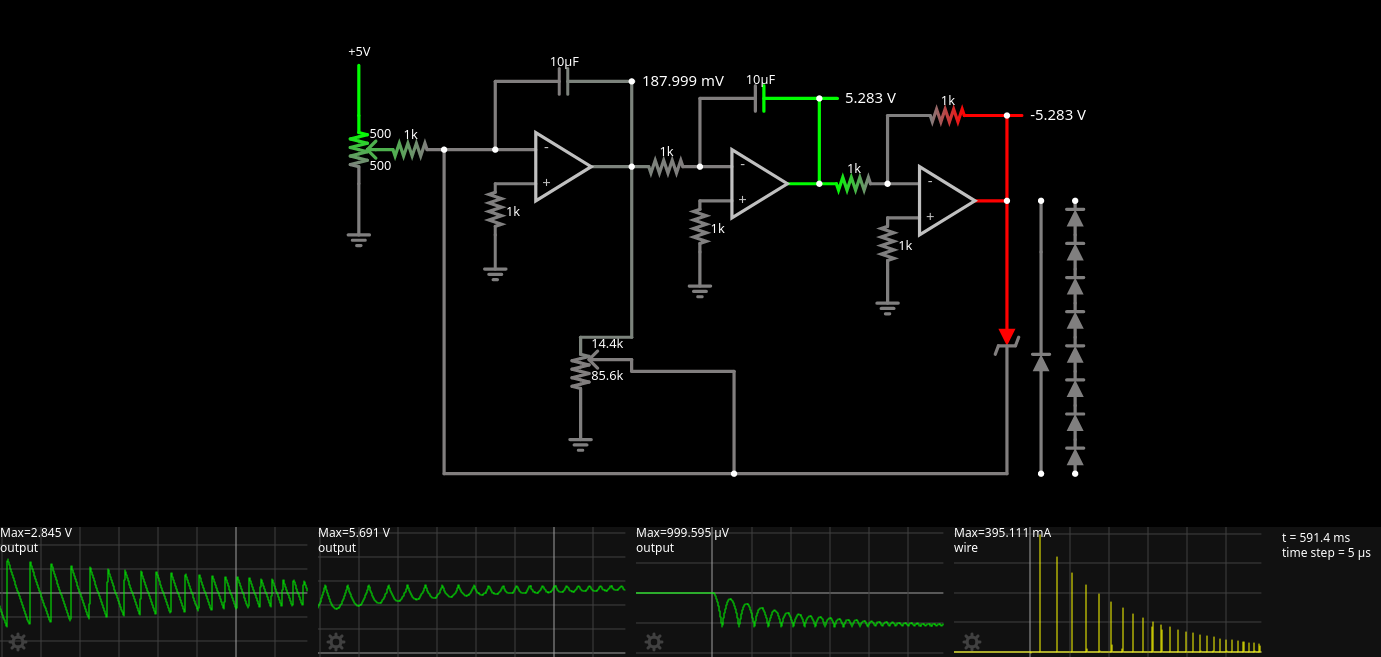
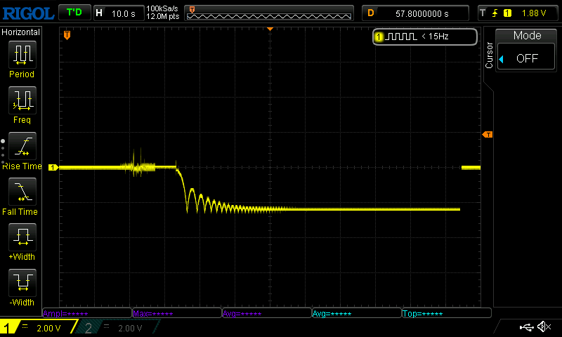
Well, things don’t always play out the same in the real world. Here’s the output of the circuit without any damping applied. As we can see, there is some damping anyway. Furthermore, the floor voltage level moves up over time, which is something I hadn’t expected.

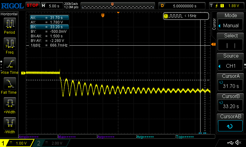
So instead of using a zener diode to set the floor, we might want to explore some other options.

1. Use an ideal diode or ideal zener diode.
2. Use some other type of diode.
3. Use a comparator to compare against a configurable floor voltage level.

Oh yeah, an ideal diode! Silly me, messing around with them non-ideal diodes. Let’s pay a couple cents more and buy some ideal ones, right?!

Enter the precision rectifier

Above, we described diodes and zener diodes as “smart wires” that become active at a certain voltage level. But that’s an “ELI5” explanation. Diodes are actually kind of devious; they do become active at a certain voltage, but when they do, they substract that voltage from the input voltage!

We could use a precision rectifier (https://en.wikipedia.org/wiki/Precision_rectifier (below circuit diagrams are taken from this page)) instead.

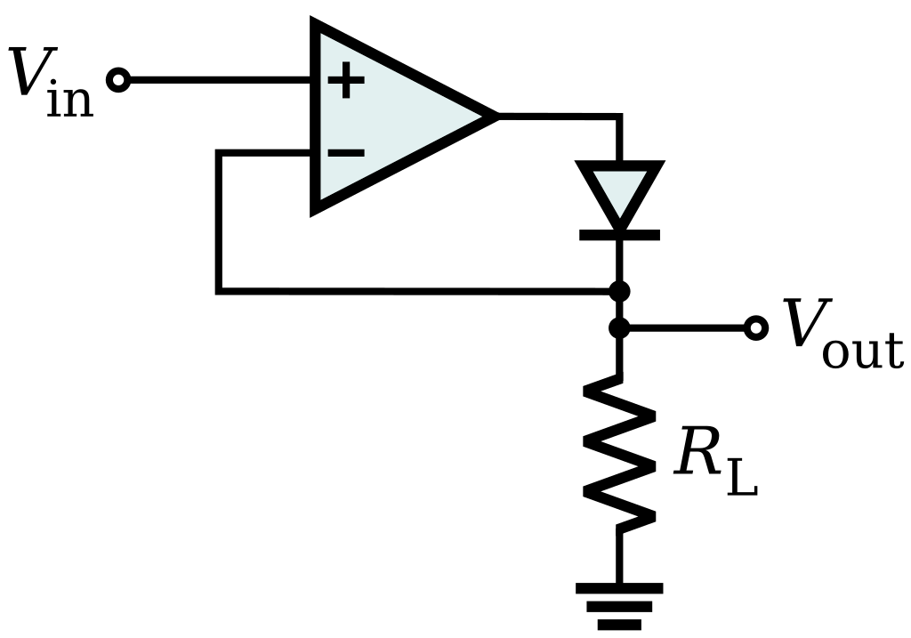
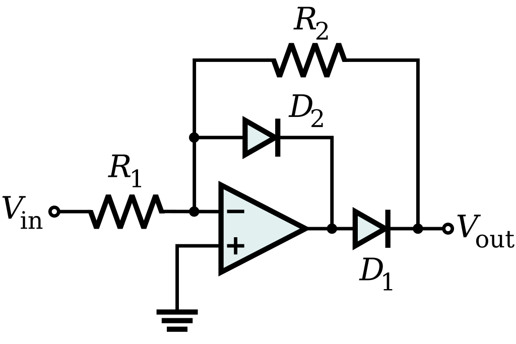
These circuits behave like diodes that don’t have a voltage drop. な、何!? Op amps, is there any thing they can’t do? There are versions that do full wave rectification too.

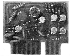
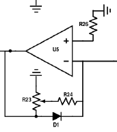
By the way, we find something close to the basic version of the precision rectifier in Mubarik Mohamoud’s circuit (page 7 of the PDF):

To be honest, using these things won’t help us much on our quest to keep things simple. We don’t need a perfect circuit; let’s use some artistic license and check out some other diodes first!

Other diodes

There are other diodes out there that have a high forward voltage. For example, how about… a white LED?!

Of course, if we wanted to be exact and stuff, we should maybe look into using comparators instead! We’ll definitely need comparators at some point so why not check them out now.

Enter the comparator

We could also use a comparator, and yes, you guessed it, our good old omnipotent friend Op Amp can be used as a comparator, because of course he (or she) can! We’ll make an op amp compare our Y coordinate voltage with a low voltage set using a potentiometer. That’s our floor.

Op amps used as comparators always output their low voltage rail or their high voltage rail, depending on whether the input voltage is lower or higher than the reference voltage. Our above op amp had 5V and -5V rails, so the comparator would output 5V or -5V. -5V is not convenient for what we’ll do later, so we’ll convert -5V to 0V by feeding the output to a diode. The negative voltage won’t make it through, only the positive 5V. Because the negative voltage won’t make it through, it will be like the input is floating. We will add a pull-down resistor.

To make our comparators actually do stuff, we can use relays. (We could use many other things, the most simple/convenient of which might be a CD4016 or similar, but the original Tennis for Two used relays, so we will too!)

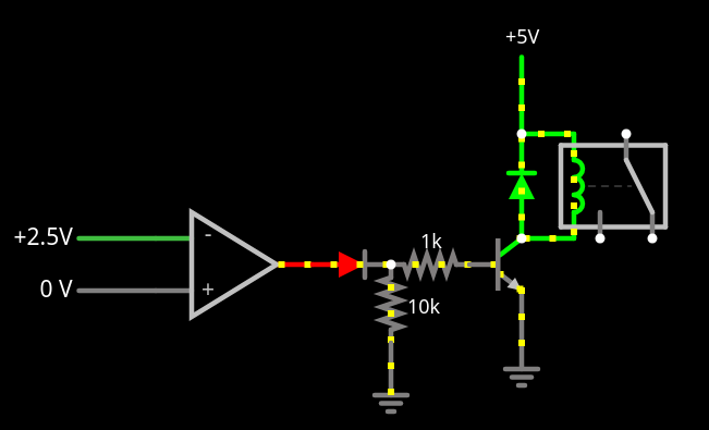
How do we connect our relay to an op amp output? Well, op amps don’t like to drive heavy loads, so we’ll use a transistor (commonly, S8050 or 2N2222), like in the following circuit. (I’m not sure if the op amps of old were able to drive relays.)

We’d like the ball to do something when the player presses a button. In the original(?) game (https://www.youtube.com/watch?v=s2E9iSQfGdg), the ball is able to bounce off the net in the middle, and can be hit at a configurable angle. I’d say we skip the net for now, but we should implement the button. More on that later!

For now, let’s just quickly think about what we need to make happen when a player hits the ball.

• The “gravity capacitor” keeps doing its thing at all times
• We just want to momentarily input a higher voltage into the first op amp’s input
• This voltage can be controlled using a potentiometer

We’ll talk about these potentiometers and buttons later.

The X axis

In a nice “Tennis for Two” game, players have beautiful controllers that have a button. This button changes the current direction of the ball. (Let’s define that a little more precisely: player 1 can only invert the direction of a ball flying right-to-left, and player 2 can only invert the direction of a ball flying left-to-right.)

In addition, there should be some kind of potentiometer inside the controller, allowing players to hit the ball hard or less hard.

Before we dream of making an ergonomic controller (yes yes, it should incorporate glass and steel and Nixie tubes to display the current score), let’s think about what the X axis is even supposed to look like.

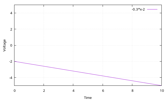
The “distance traveled” plot for the Y axis was a curve, but for the X axis, it’s a straight line. Conversely, the “velocity” plot for the Y axis was linear, but for the X axis, it’s a constant. (For illustration: in the plots below, the ball travels at a constant velocity of x volts/second.) (In reality the X axis velocity should slow down a little bit over time due to air resistance; we could model this by fudging in some kind of damping mechanism.)

The X axis circuit works like the Y axis circuit, in that it is built from op amps. However, we integrate only once. (So just a single op amp, actually.) In the Y axis, we integrated twice. (See above if you can’t remember how that worked.)

First of all, some definitions: player 1 is on the left side of the screen (where the X axis is negative), player 2 on the right side (where the X axis is positive). Here are some example graphs of the X axis:

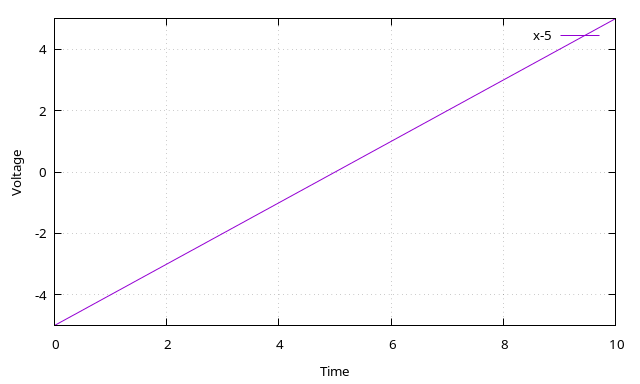
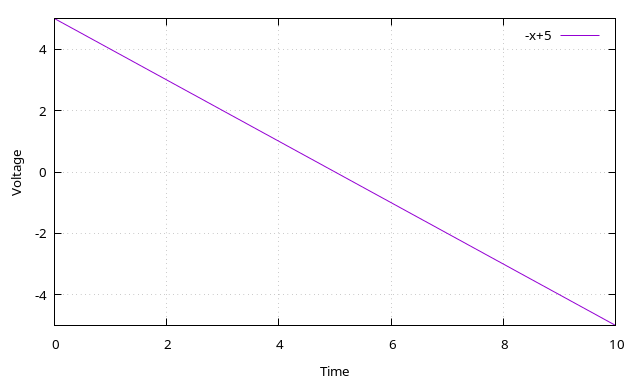
Players use a potentiometer to decide how hard the ball is hit. This potentiometer sets a voltage that represents the velocity. This voltage is connected to op amp 1.

Here’s an example of the ball being hit:

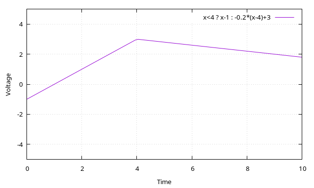
(Hey, gnuplot, it’s been a while.)

There is one minor engineering problem: as the player sets the velocity with their controller, we have to make sure they can’t change the velocity after hitting the ball. If we just hooked up the potentiometer directly to the first stage op amp, the player could/would make the ball slower or faster in mid-air by fiddling with their potentiometer after hitting the ball. Not very tennis-like!

How can we do this? Well, there should be a momentary push button. If this button is pushed, there should be a check to see if we are on the correct half of the screen, and if the ball is traveling in the correct direction. This is implemented using comparators and AND circuits. If the checks pass, we apply the voltage set by the potentiometer to feed op amp 1.

• We need to check conditions. We use op amps configured as comparators. We could easily use NPN transistors to form an AND gate but we’re lazy and will use 74-series AND logic chips. (Which weren’t quite around yet when this game was invented!)
• Our comparators compare against the middle of the screen, which is 0V. This makes the wiring very easy: one input is the current voltage, and the other input is GND.
• The other player has the inputs on the comparators swapped. (I.e., “one input is GND, the other input is the current voltage”)
• One voltage is the current voltage as it is output by the X axis op amp (the absolute position of the ball on the screen), the other voltage is the voltage that is input into the op amp (i.e., the output of the sample and hold circuit mentioned below).
• After checking the conditions, the new voltage is set. This immediately changes the ball’s direction, which means that the conditions are no longer true after a very short moment.
• However, we need to keep applying the same voltage until the other player presses their button.
• We can store the potentiometer voltage in a sample and hold circuit.

Sample and hold circuit

Well, apparently there are many ways to build a sample and hold circuit. I happen to have a (Japanese) book called 回路の素 101 that has a whole bunch of analog circuits, many of them using op amps, and among those, two circuits to do sample and hold.

Here are the two circuits in a simulator:

We can see that this circuit only holds the sampled value for a few milliseconds. The charging of the capacitor is slow, and it discharges itself pretty quickly.

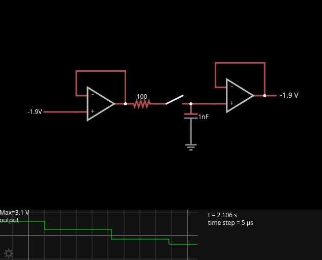
In real life, I went for a 1 uF capacitor, for improved debuggability: when using an oscilloscope (or even multimeter) to make sure that your capacitor is holding the expected voltage, you will find that the voltage drops very quickly. This is due to the oscilloscope’s input impedance, which is likely 1 MΩ. Using a tiny capacitor, the voltage will be gone almost immediately. Using a 1 uF capacitor, you have a couple seconds.

“Controllers”

The controllers are conveniently placed on a hard to reach corner on the breadboard. We have two potentiometers and one button per player. When the button is pressed and the comparators’ outputs going to the AND chip look good, we drive an SPDT relay. SPDT means that the relay normally connects player 2’s potentiometer to the input of the sample and hold circuit. But when the relay is active, it instead connects player 1’s potentiometer to the input of the sample and hold circuit. (Or the other way round, it doesn’t matter much.)

The sample and hold circuit must hold a new value when either player 1 or player 2 presses their button (and the abovementioned conditions pass). This means that we need an OR circuit as well.

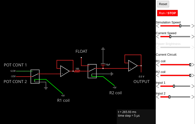
Outside the controller, we have a circuit that is inserted into the aforementioned sample and hold ciruit, as shown below. “Input 1” and “Input 2” are directly attached to the potentiometer outputs. The “R1 coil” (relay 1 coil) and “R2 coil” inputs are the binary signals mentioned above.

Here’s a schematic of this sub-circuit:

Other implementation notes

I used a 74LS08 chip for the AND gates. I’m using all four. I used a 74LS02 chip for the OR gate. This is a NOR chip, and I’m using two NOR gates to emulate one OR gate. The remaining two NOR gates are currently not used. These logic chips could be replaced with BJTs if you want to make the whole thing more era-appropriate, but you might find that the naive AND/OR gate implementations are a bit janky.

There is a lot of space between the “sample and hold” op amp and the “comparator” op amps. I added an op amp I didn’t need!

Putting it all together

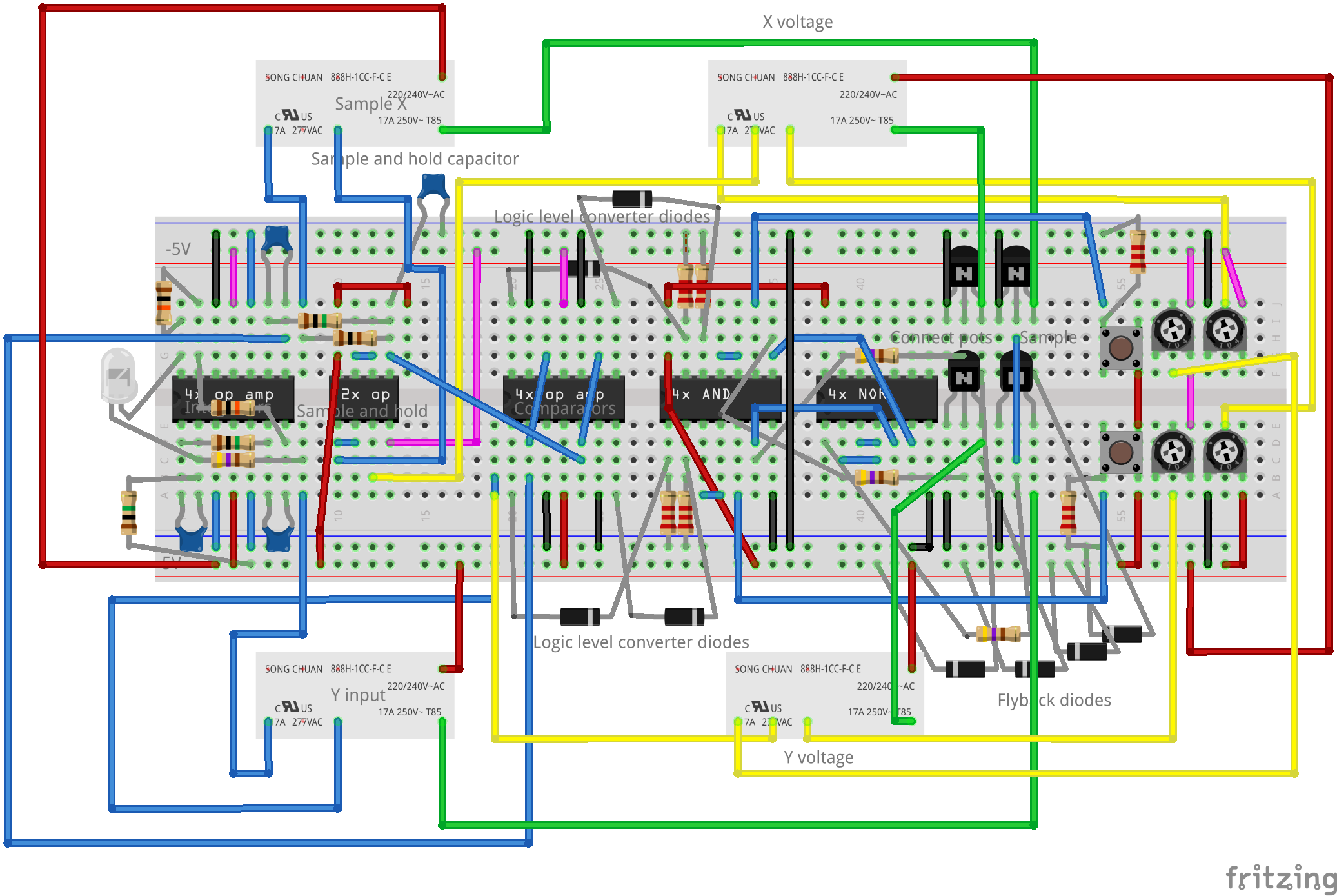
I decided to squeeze everything onto a single breadboard. To make this a little easier, I decided to build the circuit in Fritzing before building it in real life.

Change history:
2024-08-05 Initial upload (“v2”)
Notes:
The relays may not be connected correctly here — some things may not make sense (e.g. X and Y could be the wrong way round, or player 1’s potentiometer could be wired to player 2’s comparators, etc.)
The relays shown in Fritzing (and thus the above image) aren’t the actual relays used. (Actual relays used are Omron G2R-1 5V relays. These don’t fit on breadboards, but we didn’t really have any space remaining on the breadboard anyway.)
The real-life version (as seen in the picture/videos below) uses two dual op amps in the “sample and hold” region, though one is not required. There might be issues in this area.
Red means a connection to +5V, purple means connection to -5V, black means connection to GND, green means connection from transistor to relay, yellow means connection from relay to somewhere on the breadboard, blue means “other connection” on the breadboard. I mostly tried to follow this rule when building the real thing, but 1) my connections from board to relay are random, 2) connections from power supply to board are all black, 3) the white wire sticking out to the right is GND and should be black.
You don’t have to use LM324s and LM358s. It’s just that I had a bunch of these lying around, waiting to be used.

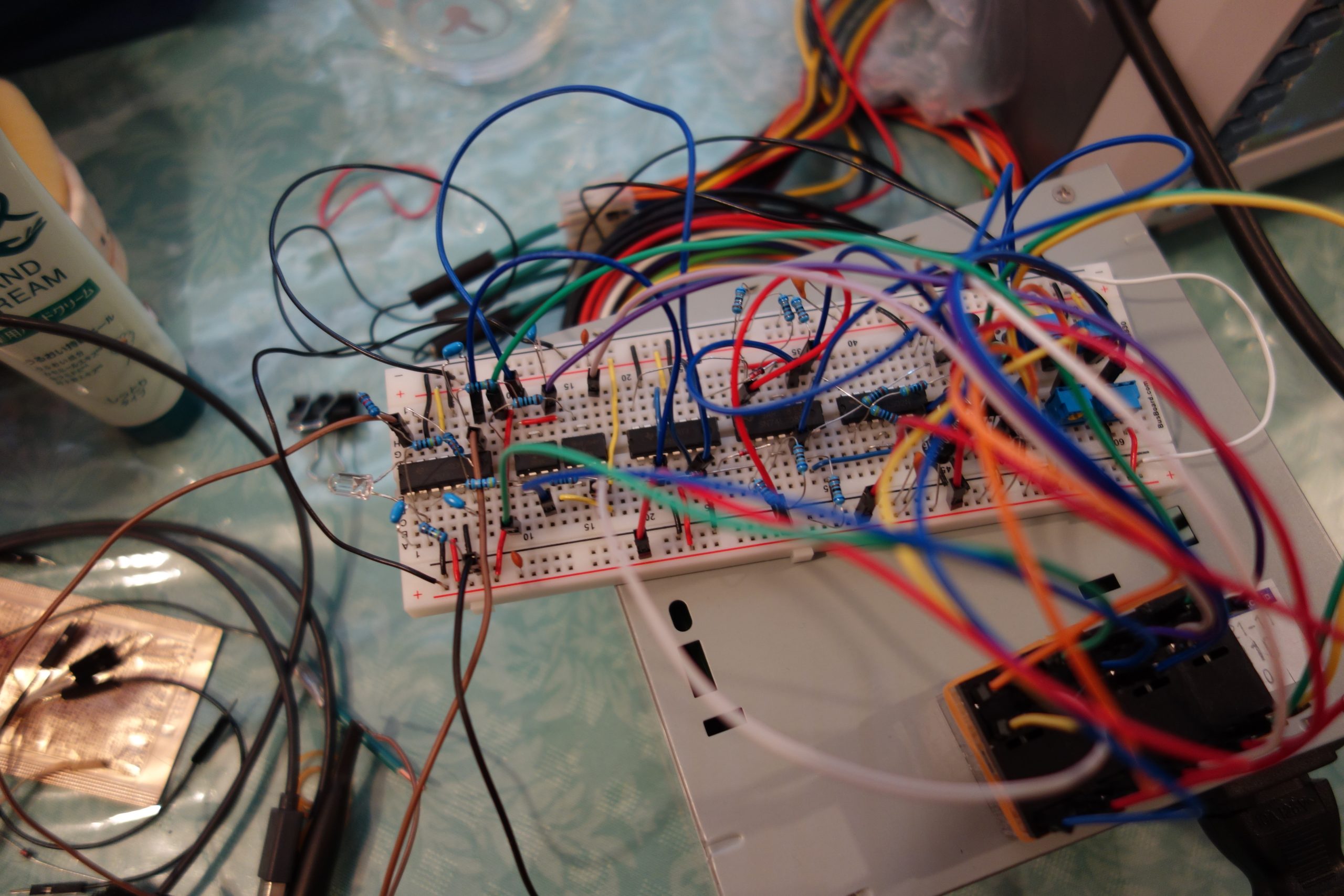
Pics/videos

Taking things further

Here is a list of features that might be pleasant to have:

• Proper controllers
• A ceiling to bounce off of (I think this is just one extra diode). Should look better than a flat line when the ball hits the -5/+5V limits!
• A nicer-looking ball
• Some audio feedback (I thought the relays would provide this, but they’re relatively quiet, actually)
• A net in the middle (both visually and functionally)
• A way to detect if a player misses
• Perform some game-like action when a player misses
• A score counter

I think you’d need another breadboard to add all this!

I think I’ve had enough of this stuff for now.